A few years ago—back in high school—I spent a little while writing programs to automatically generate mazes. It was a fun exercise and helped me come to grips with recursion: the first time I implemented it (in Java), I couldn’t get the recursive version to work properly so ended up using a while loop with an explicit stack!
Making random mazes is actually a really good programming exercise: it’s relatively simple, produces cool pictures and does a good job of covering graph algorithms. It’s especially interesting for functional programming because it relies on graphs and randomness, two things generally viewed as tricky in a functional style.
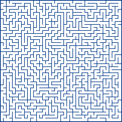
So lets look at how to implement a maze generator in Haskell using inductive graphs for our graph traversal. Here’s what we’re aiming for:
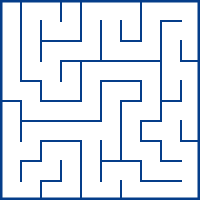
A simple maze built from a grid.
Inductive graphs are provided by Haskell’s “Functional Graph Library” fgl.
All of the code associated with this post is up on GitHub so you can load it into GHCi and follow along. It’s also a good starting point if you want to hack together your own mazes later on. It’s all under a BSD3 license, so you can use it however you like.
The Algorithm
We can generate a perfect maze by starting with a graph representing a grid and generating a random spanning tree. A perfect maze has exactly one path between any two points—no cycles or walled-off areas. A spanning tree of a graph is a tree that connects every single node in the graph.
There are multiple algorithms we can use to generate such a tree. Let’s focus on the simplest one which is just a randomized depth first search (DFS):
start with a grid that has every possible wall filled in
choose a cell to begin
from your current cell, choose a random neighbor that you haven’t visited yet
move to the chosen neighbor, knocking down the wall between it
if there are no unvisited neighbors, backtrack to the previous cell you were in and repeat
otherwise, repeat from your new cell
Our algorithm starts with a grid and produces a maze by deleting walls.
Inductive Data Types
To write our DFS, we need some way to represent a graph. Unfortunately, graphs are often inconvenient functional languages: standard representations like adjacency matrices or adjacency lists were designed with an imperative mindset. While you can certainly use them in Haskell, the resulting code would be relatively awkward.
But what sorts of structures does Haskell handle really well? Trees and lists come to mind: we can write very natural code by pattern matching. A very common pattern is to inspect a list as a head element and a tail, recursing on the tail:
foo (x:xs) = bar x : foo xs
Exactly the same pattern is useful for trees where we recurse on the children of a node:
foo (Node x children) =Node (bar x) (map foo children)
This pattern of choosing a “first” element and then recursing on the “rest” of the structure is extremely powerful. I like to think of it as “layering” your computation on the “shape” of the data structure.
We can decompose lists and trees like this very naturally because that’s exactly how they’re constructed in the first place: pattern matching is just the inverse of using the constructor normally. Even the syntax is the same! The pattern (x:xs) decomposes the result of the expression (x:xs). And since we’re just following the inherent structure of the type, there is always exactly one way to break the type apart.
These sorts of types are called inductive data types by analogy to mathematical induction. Generally, they have two branches: a base case and a recursive case—just like a proof by induction! Consider a List type:
dataList a =Empty-- base case|Cons a (List a) -- inductive case
Pretty straightforward.
Unfortunately, graphs don’t have this same structure. A graph is defined by its set of nodes and edges—the nodes and edges do not have any particular order. We can’t build a graph in a unique way by adding on nodes and edges because any given graph could be built up in multiple different ways. And so we can’t break the graph up in a unique way. We can’t pattern match on the graph. Our code is awkward.
Inductive Graphs
Inductive graphs are graphs that we can view as if they were a normal inductive data type. We can split a graph up and recurse over it, but this isn’t a structural operation like it would be for lists and, more importantly, it is not canonical: at any point, many different graph decompositions might make sense.
We can always view a graph as either empty or as some node, its edges and the rest of the graph. A node together with its incoming and outgoing edges is called a context; the idea is that we can split a graph up into a context and everything else, just like we can split a list up into its head element and everything else.
Conceptually, this is as if we defined a graph using two constructors, Empty and :& (in infix syntax):
The actual graph view in fgl is a bit different and supports node and edge labels, which I’ve left out for simplicity. The fundamental ideas are the same.
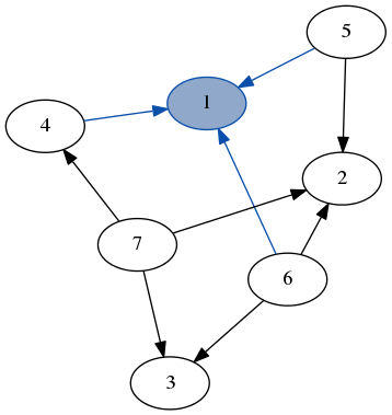
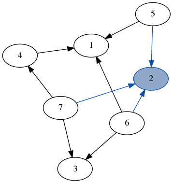
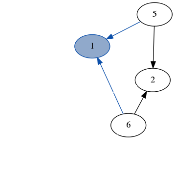
Consider a small example graph:
Just a random graph.
We could decompose this graph into the node 1, its context and the rest of the graph:
(Context [4,5,6] 1 []) :& graph our graph decomposed into the node 1, its edges to 4, 5 and 6 as well as the rest of the graph.
However, we could just as easily decompose the same example graph into node 2 and the rest:
(Context [5,6,7] 2 []) :& graph another equally valid way to decompose the same graph.
This means we can’t use this algebraic definition directly. Instead the actual graph type is abstract and we just view it using contexts, like above. Unlike normal pattern matching, viewing an abstract type is not necessarily the inverse of constructing it.
We accomplish this by using a matching function that takes a graph and returns a context decomposition. Since there is no “natural” first node to return, the simplest matching function matchAny returns an arbitrary (implementation defined) decomposition:
matchAny ::Graph-> (Context, Graph)
In fgl, Context is just a tuple with four elements: incoming edges, the node, the node label and outgoing edges.
The simplest way to use matchAny is with a case expression. Here’s the moral equivalent of head for graphs:
Pattern matching with case like this is a bit awkward. Happily, we can get much nicer syntax using ViewPatterns, which allow us to call functions inside a pattern. Here’s a prettier version of ghead which does exactly the same thing:
All my functions from now on will use ViewPatterns because they lead to nicer, more compact and more readable code.
Since the exact node that matchAny returns is implementation defined, it’s often inconvenient. We can overcome this using match, which matches a specific node.
match ::Node->Graph-> (MaybeContext, Graph)
If the node is not in the graph, we get a Nothing for our context. This function can also be used as a view pattern:
foo (match node -> (Just context, graph)) =...
This makes it easy to do directed traversals of the graph: we can “travel” to the node of our choice.
A Real Example
All functions in fgl are actually specified against a Graph typeclasses rather than a concrete implementation. This typeclass mechanism is great since it allows multiple implementations of inductive graphs. Unfortunately, it also breaks type inference in ways that are sometimes hard to track down so, for simplicity, we’ll just use the provided implementation: Gr. Gr n e is a graph that has nodes labeled with n and edges labeled with e.
Map
The “Hello, World!” of recursive list functions is map, so lets start by looking at a version of map for graphs. The idea is to apply a function to every node label in the graph.
For reference, here’s list map:
map :: (a -> b) -> [a] -> [b]map f [] = []map f (x:xs) = f x :map f xs
First, we have a base case for the empty list. Then we decompose the list, apply the function to the single element and recurse on the remainder.
The map function for graph nodes looks very similar:
mapNodes :: (n -> n') ->Gr n e ->Gr n' emapNodes _ g | Graph.isEmpty g = Graph.emptymapNodes f (matchAny -> ((in', node, label, out), g)) = (in', node, f label, out) & mapNodes f g
The base case is almost exactly the same. For the recursive case, we use matchAny to decompose the graph into some node and the rest of the graph. For the node, we actually get a Context which contains the incoming edges (in'), outgoing edges (out), the node itself (node) as well as the label (label). We just want to apply a function to the label, so we pass the rest of the context through unchanged. Finally, we recombine the graph with the & function, which is the graph equivalent of : for lists. (Although note that it is not a constructor but just a function!)
Since we used matchAny, the exact order we map over the graph is not defined! Apart from that, the code feels very similar to programming against normal Haskell data types and characterizes fgl in general pretty well.
DFS
Our maze algorithm is going to be a randomized depth-first search. We can first write a simple, non-random DFS and then go from that to our maze algorithm. That’s one of my favorite ways to implement more difficult algorithms: start with something really simple and iterate.
The basic DFS is actually pretty similar to mapNodes except that we’re going to build up a list of visited nodes as we go along instead of building a new graph. It’s also a directed traversal unlike the undirected map.
The first version of our DFS will take a graph and traverse it starting from a given node, returning a list of the nodes visited in order. Here’s the code:
dfs ::Graph.Node->Gr a b -> [Node]dfs start graph = go [start] graphwhere go [] _ = [] go _ g | Graph.isEmpty g = [] go (n:ns) (match n -> (Just c, g)) = n : go (Graph.neighbors' c ++ ns) g go (_:ns) = go ns g
The core logic is in the helper go function. It takes two arguments: a list, which is the stack of nodes to visit, and the remainder of the graph.
The first two lines of go are the base cases. If we either don’t have any more nodes on the stack or we’ve run out of nodes in the graph, we’re done.
The recursive cases are more interesting. First, we get the node we want to visit (n) from our stack. Then, we use that to direct our match with the match n function. If this succeeds, we add n to our result list and push every neighbor of n to the stack. If the match failed, it means we visited that node already, so we just ignore it and recurse on the rest of the stack.
We find the neighbors of a node using the neighbors' function which gets the neighbors of a context. In fgl, functions named with a ' typically act on contexts.
The important idea here is that we don’t need to explicitly keep track of which nodes we’ve visited—after we visit a node, we always recurse on the rest of the graph which does not contain it. This sort of behavior is common to a bunch of different graph algorithms making this a very useful pattern.
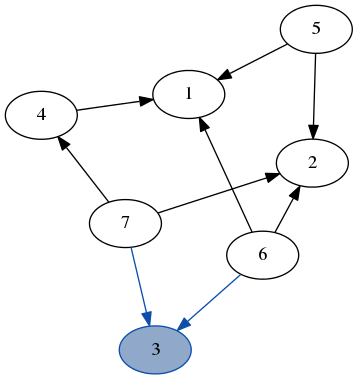
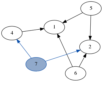
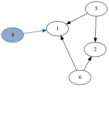
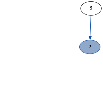
Here’s a quick demo of dfs running over the example graph from earlier. Note how we don’t need to keep track of which nodes we’ve visited because we always recurse on the part of the graph that only has unvisited nodes.
stack: [7, 6]
result: [3]
stack: [4, 2, 6]
result: [3, 7]
stack: [1, 2, 6]
result: [3, 7, 4]
stack: [6, 5, 2, 6]
result: [3, 7, 4, 1]
stack: [2, 5, 2, 6]
result: [3, 7, 4, 1, 6]
stack: [5, 5, 2, 6]
result: [3, 7, 4, 1, 6, 2]
stack: [5, 2, 6]
result: [3, 7, 4, 1, 6, 2, 5]
Often—like for generating mazes—we don’t care about which node to start from. This is where ghead comes in since it selects an arbitrary node for us! The only thing to consider is that ghead will fail on an empty graph.
EDFS
dfs gives us nodes in the order that they were visited. But for mazes, we really care about the edges we followed rather than just nodes. So lets modify our dfs into an edfs which returns a list of edges rather than a list of nodes. In fgl, an edge is just a tuple of two nodes: (Node, Node).
The modifications from our original dfs are actually quite slight: we keep a stack of edges instead of a stack of nodes. This requires modifying our starting condition:
Since we’re storing edges on our stack, we can’t just put the start node directly on there. Instead, we just match on it and start with its edges on the stack.
We need the extra call to normalize because we’re treating our edges as if they were undirected and we need to make sure that the two nodes that define an edge always appear in the same order. It just goes through the edges and swaps the nodes if they’re in the wrong order.
The other change was for the recursive case, where we push edges onto the stack instead of nodes:
go ((p, n) : ns) (match n -> (Just c, g)) =
    (p, n) : go (neighborEdges' c ++ ns) g
neighborEdges is just a helper function that returns all the incoming and outgoing edges from a context. (In the actual code, I called it lNeighbors because it actually returns labeled edges.
Randomness
The final change we need to generate a maze is adding randomness. We want to shuffle the list of neighboring edges before putting it on the stack. We’re going to use the MonadRandom class, which is compatible with a bunch of other monads like IO. I wrote a naïve O(n²) shuffle:
shuffle ::MonadRandom m => [a] -> m [a]
Given this, we just need to modify edfs to use it which requires lifting everything into the monad.
edfsR ::MonadRandom m =>Graph.Node->Gr n e -> m [(Node, Node)]edfsR start (match start -> (Just ctx, graph)) = liftM normalize $ go (lNeighbors' ctx) graphwhere go [] _ =return [] go _ g | Graph.isEmpty g =return [] go ((p, n):ns) (match n -> (Just c, g)) =do edges <- shuffle $ neighborEdges' c liftM ((p, n) :) $ go (edges ++ ns) g go (_:ns) g = go ns g
The differences are largely simple and very type-directed: you have to add some calls to return and liftM, but you get some nice type errors that tell you where to add them. The only other change is using shuffle which is straightforward with do-notation.
For something that’s supposed to be awkward in functional programming, I think the code is actually pretty neat and easy to follow!
Since we used the MonadRandom class, we can use edfsR with any type that provides randomness capabilities. This includes IO, so we can use it directly from GHCi, which is quite nice. We could also run it in a purely deterministic way by providing a seed if we wanted.
Mazes
We have a random DFS that gives us a list of edges—the core of the maze generation algorithm. However, it’s difficult to go from a set of edges to drawing a maze. The final pieces of the puzzle are labeling the edges in a way that’s convenient to draw and generating the graph for the initial grid.
This is the first place where we’re going to use edge labels. Each edge represents a wall and we need enough information to draw it. We need to know the walls location and its orientation (either horizontal and vertical). For simplicity, we will locate the walls by the location of the cell either below or to the right of the wall as appropriate for its direction. Here are the relevant types:
dataOrientation=Horizontal|Verticalderiving (Show, Eq)dataWall=Wall (Int, Int) Orientationderiving (Show, Eq)typeGrid=Gr () Wall-- () means no node labels needed
Next, we need to build the starting graph: a maze with every single wall present. We can assemble it with the mkGraph function which takes a list of nodes and a list of edges. We want to label each edge with its location and orientation. There’s likely a better way to do all this, but for now I take advantage of the fact that Node is just an alias for Int:
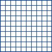
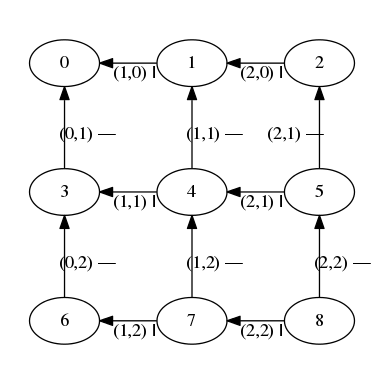
grid ::Int->Int->Gridgrid width height = Graph.mkGraph nodes edgeswhere nodes = [(node, ()) | node <- [0..width * height -1]] edges = [(n, n', wall n Vertical) | (n, _) <- nodes, (n, _) <- nodes, n - n' ==1&& n `mod` width /=0 ]++ [(n, n', wall n Horizontal) | (n,_) <- nodes, (n',_) <- nodes, n - n' == width ] wall n =let (y, x) = n `divMod` width inWall (x, y)
A 3 × 3 grid. The edges are labeled with an (x, y) position and either Horizontal (—) or Vertical (|).
Running edfsR over a starting maze will give us the list of walls that were knocked down—they’re the ones we don’t want to draw. We can easily go from this to the compliment list of walls to draw using the list different operator \\\\ from Data.List:
Since a grid is always going to have nodes, we can use ghead safely.
This produces a list of edges to draw from the graph. To actually draw them, we would start by looking their labels up in the grid and then use the position and orientation to figure out the walls’ absolute positions. (My actual implementation keeps track of edge labels as it does the DFS.)
All of the drawing code is in Draw.hs and uses cairo for the actual drawing. Cairo is a C library that provides something very similar to an HTML Canvas but for GtK; it can also output images. If you just want to play around with the mazes, you can draw one to a png with:
genPng defaults "my-maze.png"4040
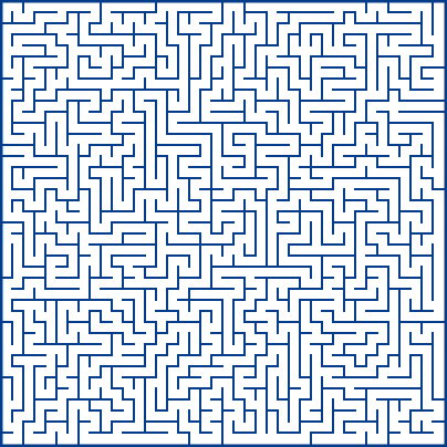
A large 40 × 40 maze with all the default drawing settings.
More Fun
We now have a basic maze generating system using inductive graphs and randomness. If you want to play around with the code a bit, there are two interesting ways to extend this code: generating mazes from other shapes and using different graph algorithms.
Other Shapes
Our system always assumes that mazes are generated from a grid of cells. However, the actual graph code doesn’t care about this at all! The grid-specific parts are just the starting graph (ie grid 40 40) and the drawing code.
A fun challenge is to look at what mazes over other sorts of graphs look like. Try writing a maze generator based on tiled hexagons, polar rectangles or even arbitrary (maybe random?) plane tilings. Or try to generate mazes in 3D!
Other Algorithms
Apart from modifying the graph, we can also modify our traversal. Play around with the DFS code: for example, you can substitute in a biased shuffle and get other shapes of mazes. If you make the shuffle more likely to choose horizontal walls than vertical ones, you will get a maze with longer vertical passages and shorter horizontal ones. How else can you change the DFS?
Randomized DFS is a nice algorithm for generating mazes because it’s simple and produces aesthetically pleasant mazes. But it’s not the only possible algorithm. You could take some other algorithms that produce spanning trees and randomize those.
One particular trick is to take an algorithm for generating minimum spanning trees, and apply it to a graph with random edge weights. The two common minimum spanning tree algorithms are Prim’s algorithm and Kruskal’s algorithm—implementing those is a good Haskell exercise and will produce subtly different looking mazes. Take a look through Minimum Spanning Tree Algorithms on Wikipedia for more inspiration.
I think this code is a great example of how, once you’ve learned a bit, many tasks in functional programming are easier than they may seem at first. Starting from the right abstractions, working with graphs or randomness need not be difficult, even in a purely functional language like Haskell.
Ultimately, this is a good exercise both for becoming a better Haskell programmer and for realizing just how versatile the language can be.